MS Data
Spectrum
The most important container for raw data and peaks is MSSpectrum which we
have already worked with in the Getting Started
tutorial. MSSpectrum is a container for 1-dimensional peak data (a
container of Peak1D). You can access these objects directly, however it is
faster to use the get_peaks() and set_peaks functions which use Python
numpy arrays for raw data access. Meta-data is accessible through inheritance
of the SpectrumSettings objects which handles meta data of a spectrum.
In the following example program, a MSSpectrum is filled with peaks, sorted according to mass-to-charge ratio and a selection of peak positions is displayed.
First we create a spectrum and insert peaks with descending mass-to-charge ratios:
1 2 3 4 5 6 7 8 9 10 11 12 13 14 15 16 17 18 19 | from pyopenms import *
spectrum = MSSpectrum()
mz = range(1500, 500, -100)
i = [0 for mass in mz]
spectrum.set_peaks([mz, i])
# Sort the peaks according to ascending mass-to-charge ratio
spectrum.sortByPosition()
# Iterate over spectrum of those peaks
for p in spectrum:
print(p.getMZ(), p.getIntensity())
# More efficient peak access with get_peaks()
for mz, i in zip(*spectrum.get_peaks()):
print(mz, i)
# Access a peak by index
print(spectrum[2].getMZ(), spectrum[2].getIntensity())
|
Note how lines 11-12 (as well as line 19) use the direct access to the
Peak1D objects (explicit iteration through the MSSpectrum object, which
is convenient but slow since a new Peak1D object needs to be created each
time) while lines 15-16 use the faster access through numpy arrays. Direct
iteration is only shown for demonstration purposes and should not be used in
production code.
To discover the full set of functionality of MSSpectrum, we use the
help() function. In particular, we find several important sets of meta
information attached to the spectrum including retention time, the ms level
(MS1, MS2, …), precursor ion, ion mobility drift time and extra data arrays.
from pyopenms import *
help(MSSpectrum)
We now set several of these properties in a current MSSpectrum:
1 2 3 4 5 6 7 8 9 10 11 12 13 14 15 16 17 18 19 20 21 22 23 24 25 26 27 28 29 30 31 32 33 34 35 36 37 | from pyopenms import *
spectrum = MSSpectrum()
spectrum.setDriftTime(25) # 25 ms
spectrum.setRT(205.2) # 205.2 s
spectrum.setMSLevel(3) # MS3
p = Precursor()
p.setIsolationWindowLowerOffset(1.5)
p.setIsolationWindowUpperOffset(1.5)
p.setMZ(600) # isolation at 600 +/- 1.5 Th
p.setActivationEnergy(40) # 40 eV
p.setCharge(4) # 4+ ion
spectrum.setPrecursors( [p] )
# Add raw data to spectrum
spectrum.set_peaks( ([401.5], [900]) )
# Additional data arrays / peak annotations
fda = FloatDataArray()
fda.setName("Signal to Noise Array")
fda.push_back(15)
sda = StringDataArray()
sda.setName("Peak annotation")
sda.push_back("y15++")
spectrum.setFloatDataArrays( [fda] )
spectrum.setStringDataArrays( [sda] )
# Add spectrum to MSExperiment
exp = MSExperiment()
exp.addSpectrum(spectrum)
# Add second spectrum and store as mzML file
spectrum2 = MSSpectrum()
spectrum2.set_peaks( ([1, 2], [1, 2]) )
exp.addSpectrum(spectrum2)
MzMLFile().store("testfile.mzML", exp)
|
We have created a single spectrum on line 3 and add meta information (drift
time, retention time, MS level, precursor charge, isolation window and
activation energy) on lines 4-13. We next add actual peaks into the spectrum (a
single peak at 401.5 m/z and 900 intensity) on line 16 and on lines 19-26 add
further meta information in the form of additional data arrays for each peak
(e.g. one trace describes “Signal to Noise” for each peak and the second traces
describes the “Peak annotation”, identifying the peak at 401.5 m/z as a
doubly charged y15 ion). Finally, we add the spectrum to a MSExperiment
container on lines 29-30 and store the container in using the MzMLFile
class in a file called “testfile.mzML” on line 37. To ensure our viewer works
as expected, we add a second spectrum to the file before storing the file.
You can now open the resulting spectrum in a spectrum viewer. We use the OpenMS
viewer TOPPView (which you will get when you install OpenMS from the
official website) and look at our MS3 spectrum:
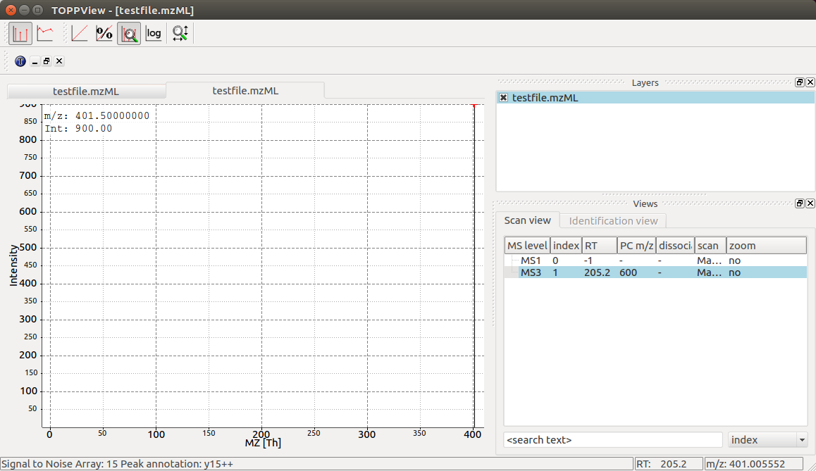
TOPPView displays our MS3 spectrum with its single peak at 401.5 m/z and it
also correctly displays its retention time at 205.2 seconds and precursor
isolation target of 600.0 m/z. Notice how TOPPView displays the information
about the S/N for the peak (S/N = 15) and its annotation as y15++ in the status
bar below when the user clicks on the peak at 401.5 m/z as shown in the
screenshot.
LC-MS/MS Experiment
In OpenMS, LC-MS/MS injections are represented as so-called peak maps (using
the MSExperiment class), which we have already encountered above. The
MSExperiment class can hold a list of MSSpectrum object (as well as a
list of MSChromatogram objects, see below). The MSExperiment object
holds such peak maps as well as meta-data about the injection. Access to
individual spectra is performed through MSExperiment.getSpectrum and
MSExperiment.getChromatogram.
In the following code, we create an MSExperiment and populate it with
several spectra:
1 2 3 4 5 6 7 8 9 10 11 12 13 14 15 16 17 18 | # The following examples creates an MSExperiment which holds six
# MSSpectrum instances.
exp = MSExperiment()
for i in range(6):
spectrum = MSSpectrum()
spectrum.setRT(i)
spectrum.setMSLevel(1)
for mz in range(500, 900, 100):
peak = Peak1D()
peak.setMZ(mz + i)
peak.setIntensity(100 - 25*abs(i-2.5) )
spectrum.push_back(peak)
exp.addSpectrum(spectrum)
# Iterate over spectra
for spectrum in exp:
for peak in spectrum:
print (spectrum.getRT(), peak.getMZ(), peak.getIntensity())
|
In the above code, we create six instances of MSSpectrum (line 4), populate
it with three peaks at 500, 900 and 100 m/z and append them to the
MSExperiment object (line 13). We can easily iterate over the spectra in
the whole experiment by using the intuitive iteration on lines 16-18 or we can
use list comprehensions to sum up intensities of all spectra that fulfill
certain conditions:
>>> # Sum intensity of all spectra between RT 2.0 and 3.0
>>> print(sum([p.getIntensity() for s in exp
...              if s.getRT() >= 2.0 and s.getRT() <= 3.0 for p in s]))
700.0
>>> 87.5 * 8
700.0
>>>
We can again store the resulting experiment containing the six spectra as mzML
using the MzMLFile object:
# Store as mzML
MzMLFile().store("testfile2.mzML", exp)
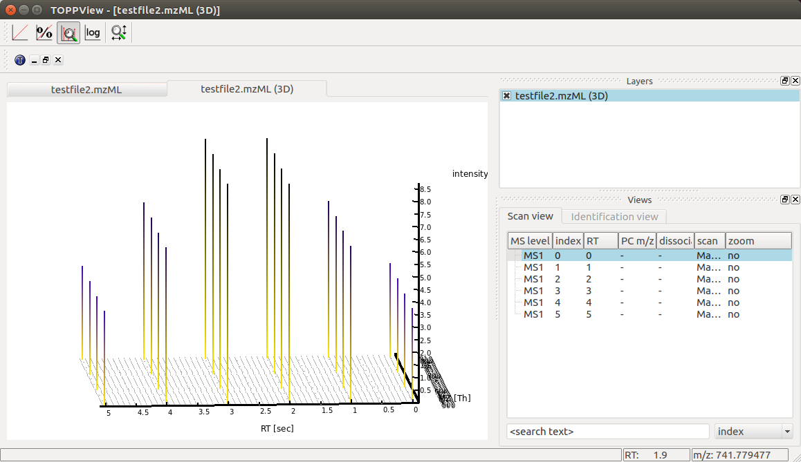
Again we can visualize the resulting data using TOPPView using its 3D
viewer capability, which shows the six scans over retention time where the
traces first increase and then decrease in intensity:
Chromatogram
An additional container for raw data is the MSChromatogram container, which
is highly analogous to the MSSpectrum container, but contains an array of
ChromatogramPeak and is derived from ChromatogramSettings:
1 2 3 4 5 6 7 8 9 10 11 12 13 14 15 16 17 18 19 20 21 22 23 24 25 26 27 | from pyopenms import *
import numpy as np
def gaussian(x, mu, sig):
return np.exp(-np.power(x - mu, 2.) / (2 * np.power(sig, 2.)))
# Create new chromatogram
chromatogram = MSChromatogram()
# Set raw data (RT and intensity)
rt = range(1500, 500, -100)
i = [gaussian(rtime, 1000, 150) for rtime in rt]
chromatogram.set_peaks([rt, i])
# Sort the peaks according to ascending retention time
chromatogram.sortByPosition()
# Iterate over chromatogram of those peaks
for p in chromatogram:
print(p.getRT(), p.getIntensity())
# More efficient peak access with get_peaks()
for rt, i in zip(*chromatogram.get_peaks()):
print(rt, i)
# Access a peak by index
print(chromatogram[2].getRT(), chromatogram[2].getIntensity())
|
We now again add meta information to the chromatogram:
1 2 3 4 5 6 7 8 9 10 11 12 13 14 15 16 17 18 19 20 21 22 | chromatogram.setNativeID("Trace XIC@405.2")
# Store a precursor ion for the chromatogram
p = Precursor()
p.setIsolationWindowLowerOffset(1.5)
p.setIsolationWindowUpperOffset(1.5)
p.setMZ(405.2) # isolation at 405.2 +/- 1.5 Th
p.setActivationEnergy(40) # 40 eV
p.setCharge(2) # 2+ ion
p.setMetaValue("description", chromatogram.getNativeID())
p.setMetaValue("peptide_sequence", chromatogram.getNativeID())
chromatogram.setPrecursor(p)
# Also store a product ion for the chromatogram (e.g. for SRM)
p = Product()
p.setMZ(603.4) # transition from 405.2 -> 603.4
chromatogram.setProduct(p)
# Store as mzML
exp = MSExperiment()
exp.addChromatogram(chromatogram)
MzMLFile().store("testfile3.mzML", exp)
|
This shows how the MSExperiment class can hold spectra as well as chromatograms.
Again we can visualize the resulting data using TOPPView using its chromatographic viewer
capability, which shows the peak over retention time:
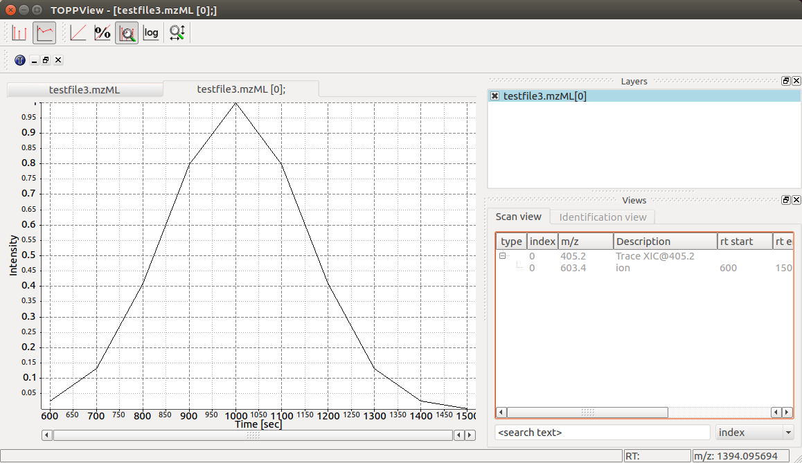
Note how the annotation using precursor and production mass of our XIC chromatogram is displayed in the viewer.