Charge and Isotope Deconvolution

A single mass spectrum contains measurements of one or more analytes and the m/z values recorded for these analytes. Most analytes produce multiple signals in the mass spectrometer, due to the natural abundance of carbon \(13\) (naturally occurring at ca. \(1\%\) frequency) and the large amount of carbon atoms in most organic molecules, most analytes produce a so-called isotopic pattern with a monoisotopic peak (all carbon are \(\ce{^{12}C}\)) and a first isotopic peak (exactly one carbon atom is a \(\ce{^{13}C}\)), a second isotopic peak (exactly two atoms are \(\ce{^{13}C}\)) etc. Note that also other elements can contribute to the isotope pattern, see the chemistry section for further details.

In addition, each analyte may appear in more than one charge state and adduct state, a singly charge analyte \(\ce{[M +H]+}\) may be accompanied by a doubly charged analyte \(\ce{[M +2H]++}\) or a sodium adduct \(\ce{[M +Na]+}\). In the case of a multiply charged peptide, the isotopic traces are spaced by PROTON_MASS / charge_state which is often close to \(0.5\ m/z\) for doubly charged analytes, \(0.33\ m/z\) for triply charged analytes etc. Note: tryptic peptides often appear at least doubly charged, while small molecules often carry a single charge but can have adducts other than hydrogen.

Single Peak Example

import pyopenms as oms

charge = 2
seq = oms.AASequence.fromString("DFPIANGER")
seq_formula = seq.getFormula() + oms.EmpiricalFormula("H" + str(charge))
isotopes = seq_formula.getIsotopeDistribution(oms.CoarseIsotopePatternGenerator(6))
print("[M+H]+ weight:", seq.getMonoWeight(oms.Residue.ResidueType.Full, 1))

# Append isotopic distribution to spectrum
s = oms.MSSpectrum()
for iso in isotopes.getContainer():
    iso.setMZ(iso.getMZ() / charge)
    s.push_back(iso)
    print("Isotope", iso.getMZ(), ":", iso.getIntensity())

oms.Deisotoper.deisotopeAndSingleChargeDefault(s, 10, True)

for p in s:
    print(p.getMZ(), p.getIntensity())

Note that the algorithm presented here as some heuristics built into it, such as assuming that the isotopic peaks will decrease after the first isotopic peak. This heuristic can be tuned by changing the parameter use_decreasing_model and start_intensity_check. In this case, the second isotopic peak is the highest in intensity and the start_intensity_check parameter needs to be set to 3.

charge = 4
seq = oms.AASequence.fromString("DFPIANGERDFPIANGERDFPIANGERDFPIANGER")
seq_formula = seq.getFormula() + oms.EmpiricalFormula("H" + str(charge))
isotopes = seq_formula.getIsotopeDistribution(oms.CoarseIsotopePatternGenerator(8))
print("[M+H]+ weight:", seq.getMonoWeight(oms.Residue.ResidueType.Full, 1))

# Append isotopic distribution to spectrum
s = oms.MSSpectrum()
for iso in isotopes.getContainer():
    iso.setMZ(iso.getMZ() / charge)
    s.push_back(iso)
    print("Isotope", iso.getMZ(), ":", iso.getIntensity())

min_charge = 1
min_isotopes = 2
max_isotopes = 10
use_decreasing_model = True
start_intensity_check = 3
oms.Deisotoper.deisotopeAndSingleCharge(
    s,
    10,
    True,
    min_charge,
    charge,
    True,
    min_isotopes,
    max_isotopes,
    True,
    True,
    True,
    use_decreasing_model,
    start_intensity_check,
    False,
)
for p in s:
    print(p.getMZ(), p.getIntensity())

Full Spectral De-Isotoping

In the following code segment, we will use a sample measurement of BSA (Bovine Serum Albumin), and apply a simple algorithm in OpenMS for “deisotoping” a mass spectrum, which means grouping peaks of the same isotopic pattern charge state:

from urllib.request import urlretrieve

gh = "https://raw.githubusercontent.com/OpenMS/pyopenms-docs/master"
urlretrieve(gh + "/src/data/BSA1.mzML", "BSA1.mzML")

e = oms.MSExperiment()
oms.MzMLFile().load("BSA1.mzML", e)
s = e[214]
s.setFloatDataArrays([])
oms.Deisotoper.deisotopeAndSingleCharge(
    s,
    0.1,
    False,
    1,
    3,
    True,
    min_isotopes,
    max_isotopes,
    True,
    True,
    True,
    use_decreasing_model,
    start_intensity_check,
    False,
)

print(e[214].size())
print(s.size())

e2 = oms.MSExperiment()
e2.addSpectrum(e[214])
oms.MzMLFile().store("BSA1_scan214_full.mzML", e2)
e2 = oms.MSExperiment()
e2.addSpectrum(s)
oms.MzMLFile().store("BSA1_scan214_deisotoped.mzML", e2)

maxvalue = max([p.getIntensity() for p in s])
for p in s:
    if p.getIntensity() > 0.25 * maxvalue:
        print(p.getMZ(), p.getIntensity())

which produces the following output

140
41

974.4572680576728 6200571.5
974.4589691256419 3215808.75

As we can see, the algorithm has reduced \(140\) peaks to \(41\) deisotoped peaks. It also has identified a molecule at \(974.45\ m/z\) as the most intense peak in the data (base peak).

Visualization

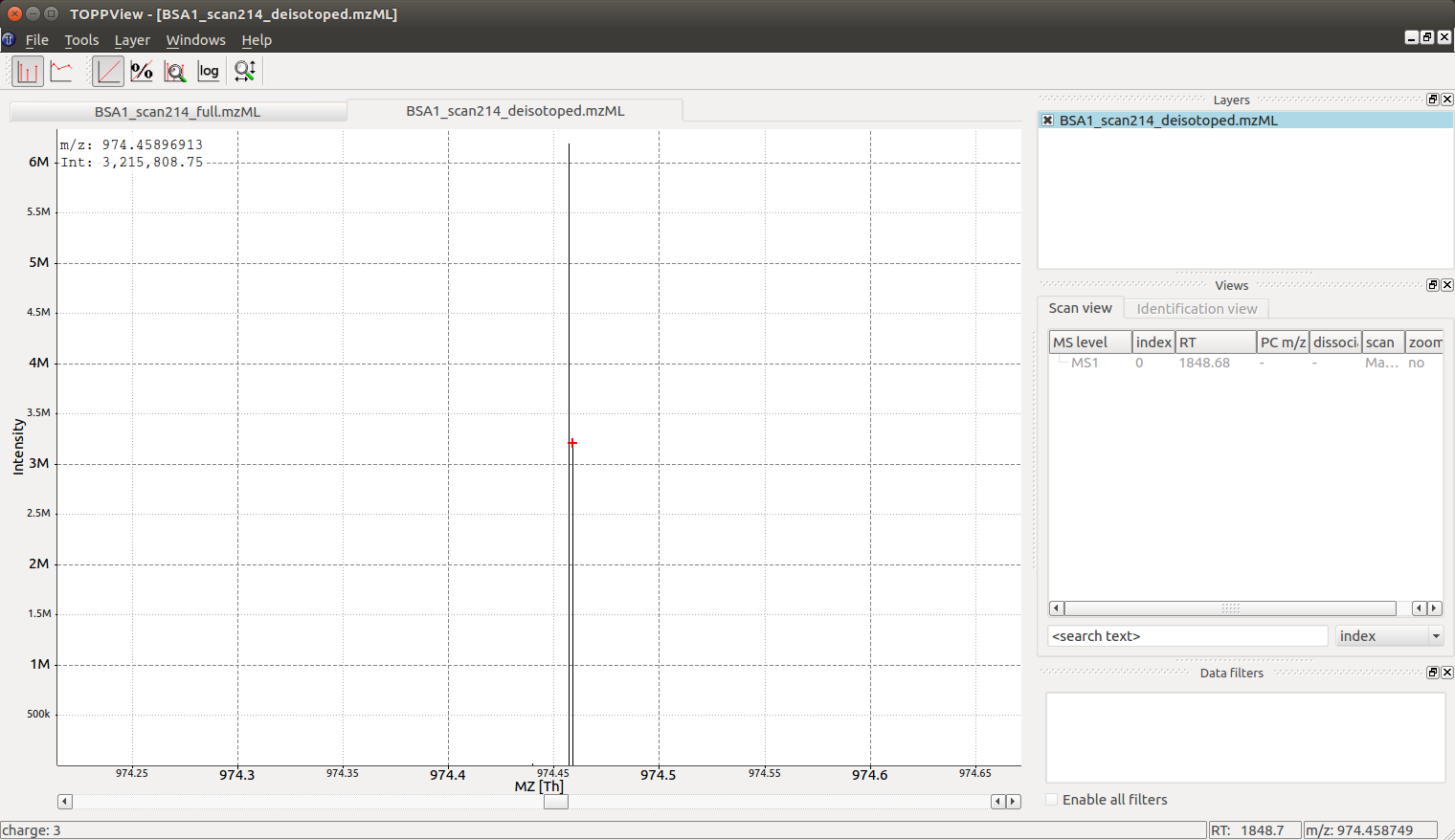
The reason we see two peaks very close together becomes apparent once we look at the data in TOPPView which indicates that the \(974.4572680576728\) peak is derived from a \(\ce{2+}\) peak at m/z \(487.73\) and the peak at \(974.4589691256419\) is derived from a \(\ce{3+}\) peak at m/z \(325.49\): the algorithm has identified a single analyte in two charge states and deconvoluted the peaks to their nominal mass of a \(\ce{[M +H]+}\) ion, which produces two peaks very close together (\(\ce{2+}\) and \(\ce{3+}\) peak):

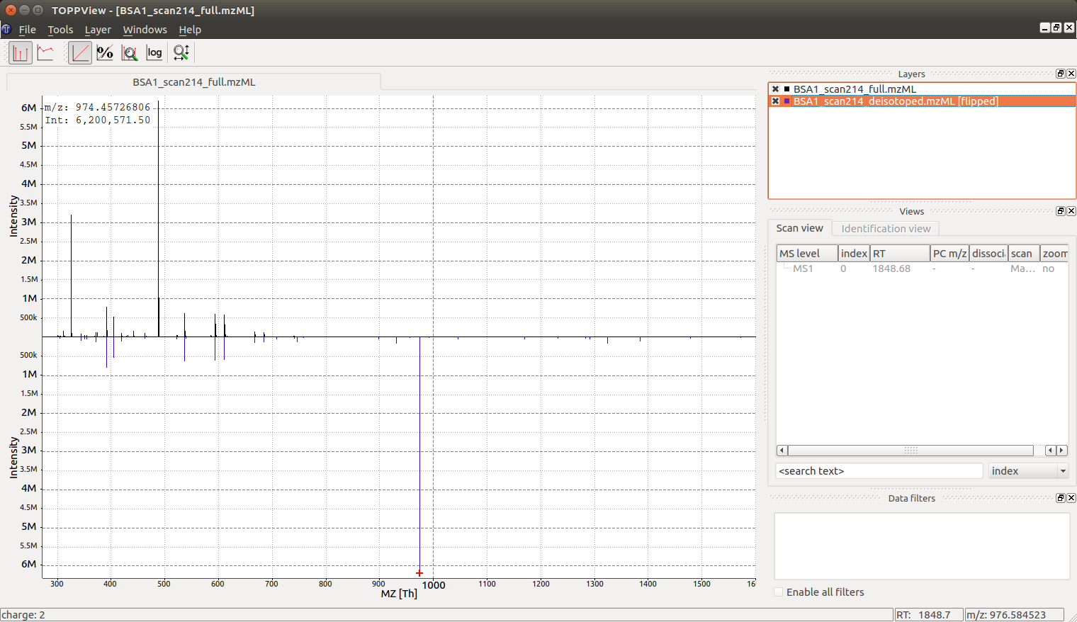
Looking at the full mass spectrum and comparing it to the original mass spectrum, we can see the original (centroided) mass spectrum on the top and the deisotoped mass spectrum on the bottom in blue. Note how hovering over a peak in the deisotoped mass spectrum indicates the charge state:

In the next section (Feature Detection), we will look at 2-dimensional deisotoping where instead of a single mass spectrum, multiple mass spectra from a LC-MS experiment are analyzed together. There algorithms analyze the full 2-dimensional (m/z and RT) signal and are generally more powerful than the 1-dimensional algorithm discussed here. However, not all data is 2 dimensional and the algorithm discussed here has many application in practice (e.g. single mass spectra, fragment ion mass spectra in DDA etc.).