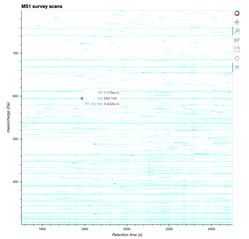
Interactive Plots

With special plotting libraries like holoviews and datashader for big data visualization as well as bokeh for interactiveness, we can use the functionality of pyOpenMS to quickly create fully interactive views of mass spectrometry data. Here we plot a full map of MS1 that can be interactively zoomed-in if you execute the code in a notebook (e.g. on Binder, see the button on top of the page).

import pyopenms as oms
import pandas as pd
import numpy as np
import datashader as ds
import holoviews as hv
import holoviews.operation.datashader as hd
from holoviews.plotting.util import process_cmap
from holoviews import opts, dim
import sys

hv.extension("bokeh")

exp = oms.MSExperiment()  # type: PeakMap
loader = oms.MzMLFile()
loadopts = loader.getOptions()  # type: PeakFileOptions
loadopts.setMSLevels([1])
loadopts.setSkipXMLChecks(True)
loadopts.setIntensity32Bit(True)
loadopts.setIntensityRange(oms.DRange1(oms.DPosition1(5000), oms.DPosition1(sys.maxsize)))
loader.setOptions(loadopts)
loader.load("../../../src/data/BSA1.mzML", exp)
exp.updateRanges()
expandcols = ["RT", "mz", "inty"]
spectraarrs2d = exp.get2DPeakDataLong(
    exp.getMinRT(), exp.getMaxRT(), exp.getMinMZ(), exp.getMaxMZ()
)
spectradf = pd.DataFrame(dict(zip(expandcols, spectraarrs2d)))
spectradf = spectradf.set_index(["RT", "mz"])

maxrt = spectradf.index.get_level_values(0).max()
minrt = spectradf.index.get_level_values(0).min()
maxmz = spectradf.index.get_level_values(1).max()
minmz = spectradf.index.get_level_values(1).min()


def new_bounds_hook(plot, elem):
    x_range = plot.state.x_range
    y_range = plot.state.y_range
    x_range.bounds = minrt, maxrt
    y_range.bounds = minmz, maxmz


points = hv.Points(
    spectradf, kdims=["RT", "mz"], vdims=["inty"], label="MS1 survey scans"
).opts(
    fontsize={"title": 16, "labels": 14, "xticks": 6, "yticks": 12},
    color=np.log(dim("int")),
    colorbar=True,
    cmap="Magma",
    width=1000,
    height=1000,
    tools=["hover"],
)

raster = (
    hd.rasterize(
        points,
        cmap=process_cmap("blues", provider="bokeh"),
        aggregator=ds.sum("inty"),
        cnorm="log",
        alpha=10,
        min_alpha=0,
    )
    .opts(active_tools=["box_zoom"], tools=["hover"], hooks=[new_bounds_hook])
    .opts(  # weird.. I have no idea why one has to do this. But with one opts you will get an error
        plot=dict(
            width=800,
            height=800,
            xlabel="Retention time (s)",
            ylabel="mass/charge (Da)",
        )
    )
)

hd.dynspread(raster, threshold=0.7, how="add", shape="square")

Result:

With this you can also easily create whole dashboards like the one hosted here on a Binder instance. If you are reading/executing this on Binder already, execute the next cell to get a link to your current instance.

import os
from IPython.display import Markdown as md

md(
    "When you are in binder already, you can quickly open the app [here]({}/msbokehapps).".format(
        os.getenv("JUPYTERHUB_SERVICE_PREFIX")
    )
)