Fragment Spectrum Generation

Generating theoretical fragment spectra is central to many identification tasks in computational mass spectrometry. TheoreticalSpectrumGenerator can be configured to generate MS2 spectra from a given peptide charge combination. There are various parameters which influence the generated ions e.g. simulating different fragmentation techniques.

Y-ion Mass Spectrum

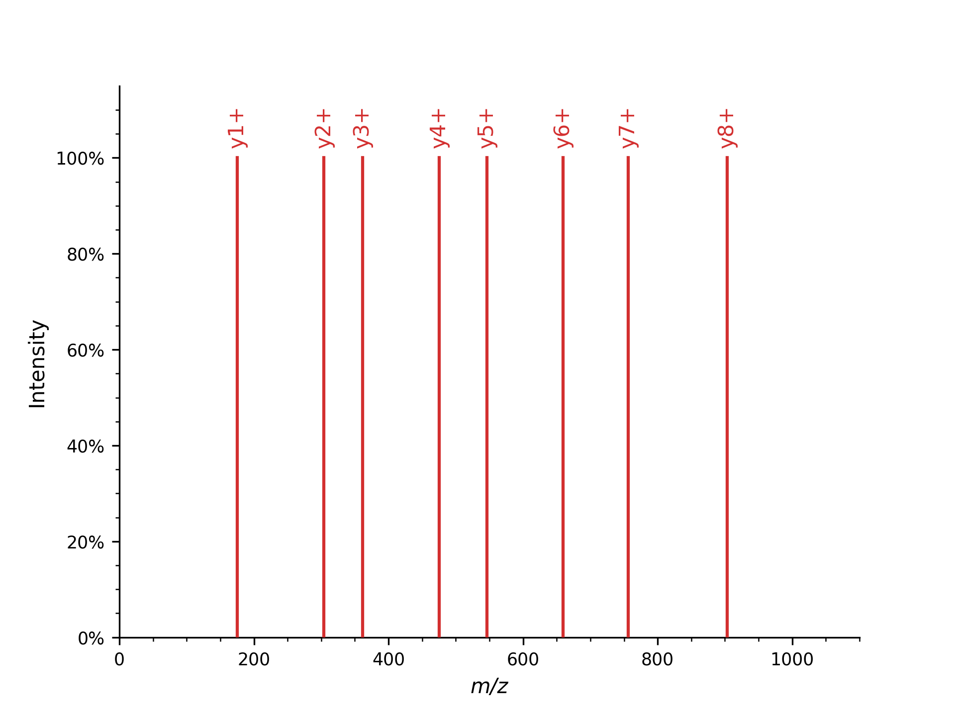
First, we will generate a simple mass spectrum that only contains y-ions

import pyopenms as oms

tsg = oms.TheoreticalSpectrumGenerator()
spec1 = oms.MSSpectrum()
peptide = oms.AASequence.fromString("DFPIANGER")
# standard behavior is adding b- and y-ions of charge 1
p = oms.Param()
p.setValue("add_b_ions", "false")
p.setValue("add_metainfo", "true")
tsg.setParameters(p)
tsg.getSpectrum(spec1, peptide, 1, 1)  # charge range 1:1

# Iterate over annotated ions and their masses
print("Spectrum 1 of", peptide, "has", spec1.size(), "peaks.")
for ion, peak in zip(spec1.getStringDataArrays()[0], spec1):
    print(ion.decode(), "is generated at m/z", peak.getMZ())

which produces all y single charged ions:

Spectrum 1 of DFPIANGER has 8 peaks.
y1+ is generated at m/z 175.118952913371
y2+ is generated at m/z 304.161547136671
y3+ is generated at m/z 361.18301123237103
y4+ is generated at m/z 475.225939423771
y5+ is generated at m/z 546.2630535832709
y6+ is generated at m/z 659.3471179341709
y7+ is generated at m/z 756.3998821574709
y8+ is generated at m/z 903.4682964445709

which you could plot with pyopenms.plotting.plot_spectrum(), automatically showing annotated ions.:

import matplotlib.pyplot as plt
from pyopenms.plotting import plot_spectrum

plot_spectrum(spec1)
plt.show()

Full Fragment Ion Mass Spectrum

We can also produce additional peaks in the fragment ion mass spectrum, such as isotopic peaks, precursor peaks, ions from higher charge states, additional ion series, or common neutral losses:

spec2 = oms.MSSpectrum()
# standard behavior is adding b- and y-ions
p2 = oms.Param()
p2.setValue("add_a_ions", "true")
# adding n-term ion (in this case, a1 and b1)
p2.setValue("add_first_prefix_ion", "true")
p2.setValue("add_precursor_peaks", "true")
# standard is to add precursor peaks with only the largest charge
p2.setValue("add_all_precursor_charges", "true")
p2.setValue("add_losses", "true")
p2.setValue("add_metainfo", "true")
tsg.setParameters(p2)
tsg.getSpectrum(spec2, peptide, 1, 2)

# Iterate over annotated ions and their masses
print("Spectrum 2 of", peptide, "has", spec2.size(), "peaks.")
for ion, peak in zip(spec2.getStringDataArrays()[0], spec2):
    print(ion.decode(), "is generated at m/z", peak.getMZ())

exp = oms.MSExperiment()
exp.addSpectrum(spec1)
exp.addSpectrum(spec2)
oms.MzMLFile().store("DFPIANGER.mzML", exp)

which outputs all 160 peaks that are generated (this is without isotopic peaks), here we will just show the first few peaks:

Spectrum 2 of DFPIANGER has 160 peaks.
a1-H2O1++ is generated at m/z 35.518008514620995
a1++ is generated at m/z 44.523291046520995
b1-H2O1++ is generated at m/z 49.515466014621
b1++ is generated at m/z 58.520748546521
y1-C1H2N1O1++ is generated at m/z 66.05629515817103
y1-C1H2N2++ is generated at m/z 67.05221565817102
a1-H2O1+ is generated at m/z 70.02874056247099
y1-H3N1++ is generated at m/z 79.54984014222102
a1+ is generated at m/z 88.03930562627099
y1++ is generated at m/z 88.06311469007102
b1-H2O1+ is generated at m/z 98.02365556247099
a2-H2O1++ is generated at m/z 109.05221565817101
b1+ is generated at m/z 116.034220626271
a2++ is generated at m/z 118.05749819007102
b2-H2O1++ is generated at m/z 123.049673158171
[...]

which you can again visualize with:

plot_spectrum(spec2, annotate_ions=False)
plt.show()

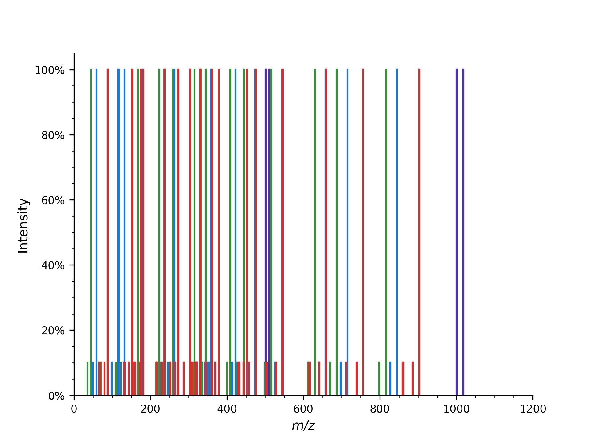
The first example shows how to put peaks of a certain type, y-ions in this case, into a mass spectrum. The second mass spectrum is filled with a complete fragment ion mass spectrum of all peaks (a-, b-, y-ions, precursor peaks, and losses).

Here, from the peptide with 9 amino acids, fragments theoretically can occur in 8 different positions, resulting in 8 peaks per ion type (a, b, and y-ion in this example code). For instance, b-ions (prefix) and y-ions (suffix) are complementary, so b3(DFP) and y6(IANGER) fragments make up the peptide “DFPIANGER.”

Adding precursor ions with the parameter add_precursor_peaks add 3 peaks with the largest charge states (precursor ion (M+H) and its loss of water ([M+H]-H2O) or ammonia ([M+H]-NH3)). To include all precursor ions with possible charge states, the add_all_precursor_charges parameter should be set to true.

The losses are based on commonly observed fragment ion losses for specific amino acids and are defined in the Residues.xml file, which means that not all fragment ions will produce all possible losses, as can be observed above: water loss is not observed for the y1 ion but for the y2 ion since glutamic acid can have a neutral water loss but arginine cannot. Similarly, only water loss and no ammonia loss is simulated in the a/b/c ion series with the first fragment capable of ammonia loss being asparagine at position 6.

The TheoreticalSpectrumGenerator has many parameters which have a detailed description located in the class documentation. Note how the add_metainfo parameter populates the StringDataArray of the output spectrum, allowing us to iterate over annotated ions and their masses.

Visualization

We can now visualize the resulting spectra using TOPPView when we open the DFPIANGER.mzML file that we produced above in TOPPView:

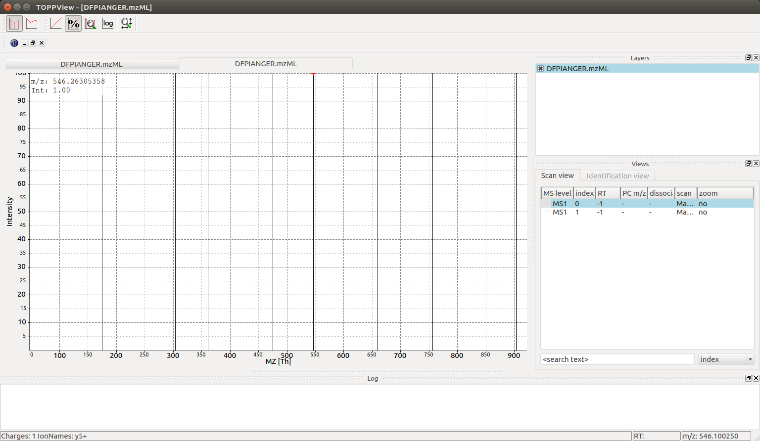
We can see all eight y ion peaks that are produced in the TheoreticalSpectrumGenerator and when we hover over one of the peaks (\(546\ mz\) in this example) there is an annotation in the bottom left corner that indicates charge state and ion name (\(\ce{y5+}\) for every peak). The larger spectrum with \(146\) peaks can also be interactively investigated with TOPPView (the second spectrum in the file):

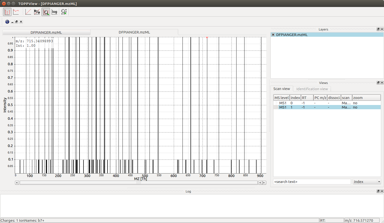
There are substantially more peaks here and the mass spectrum is much busier, with singly and double charged peaks of the b, y and a series creating \(44\) different individual fragment ion peaks as well as neutral losses adding an additional \(102\) peaks (neutral losses easily recognizable by their \(10-fold\) lower intensity in the simulated spectrum).