MS Data#
Spectrum#
The most important container for raw data and peaks is MSSpectrum which we
have already worked with in the Getting Started
tutorial. MSSpectrum is a container for 1-dimensional peak data (a
container of Peak1D). You can access these objects directly, by using an iterator or indexing.
Meta-data is accessible through inheritance of the SpectrumSettings
objects which handles meta data of a mass spectrum.
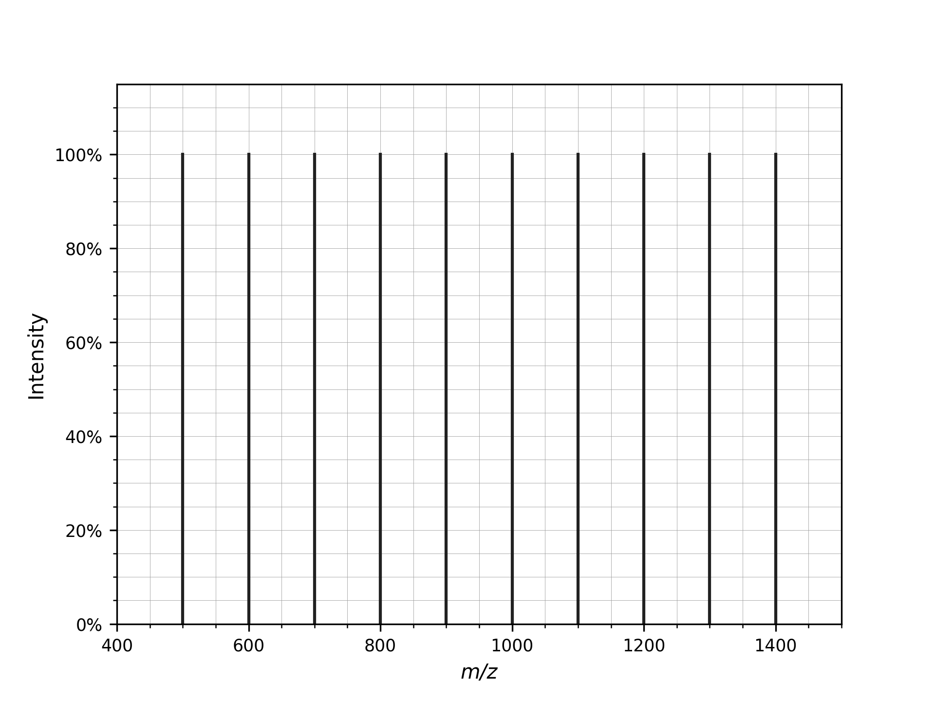
In the following example program, a MSSpectrum is filled with peaks, sorted
according to mass-to-charge ratio and a selection of peak positions is
displayed.
First we create a mass spectrum and insert peaks with descending mass-to-charge ratios:
 1import pyopenms as oms
 2
 3spectrum = oms.MSSpectrum()
 4mz = range(500, 1500, 100)
 5i = [1 for mass in mz]
 6spectrum.set_peaks([mz, i])
 7
 8# Sort the peaks according to ascending mass-to-charge ratio
 9spectrum.sortByPosition()
10
11# Iterate over spectrum of those peaks
12for p in spectrum:
13    print(p.getMZ(), p.getIntensity())
14
15# Access a peak by index
16print("\nFirst peak: ", spectrum[0].getMZ(), spectrum[0].getIntensity())
500.0 1.0
600.0 1.0
700.0 1.0
800.0 1.0
900.0 1.0
1000.0 1.0
1100.0 1.0
1200.0 1.0
1300.0 1.0
1400.0 1.0

First peak: 500.0 1.0
Note how lines 12-13 (as well as line 16) use the direct access to the
Peak1D objects (explicit iteration through the MSSpectrum object, which
is convenient but slow since a new Peak1D object needs to be created each
time).
The following example uses the faster access through numpy arrays with get_peaks() or
set_peaks(). Direct iteration is only shown for demonstration purposes and should not be used in
production code.
1# More efficient peak access with get_peaks()
2for mz, i in zip(*spectrum.get_peaks()):
3    print(mz, i)
500.0 1.0
600.0 1.0
700.0 1.0
800.0 1.0
900.0 1.0
1000.0 1.0
1100.0 1.0
1200.0 1.0
1300.0 1.0
1400.0 1.0
To discover the full set of functionality of MSSpectrum, we use the Python
help() function. In particular, we find several important sets of meta
information attached to the mass spectrum including retention time, the MS level
(MS1, MS2, …), precursor ion, ion mobility drift time and extra data arrays.
1help(oms.MSSpectrum)
We now set several of these properties in a current MSSpectrum:
 1# create spectrum and set properties
 2spectrum = oms.MSSpectrum()
 3spectrum.setDriftTime(25)  # 25 ms
 4spectrum.setRT(205.2)  # 205.2 s
 5spectrum.setMSLevel(3)  # MS3
 6
 7# Add peak(s) to spectrum
 8spectrum.set_peaks(([401.5], [900]))
 9
10# create precursor information
11p = oms.Precursor()
12p.setMZ(600)  # isolation at 600 +/- 1.5 Th
13p.setIsolationWindowLowerOffset(1.5)
14p.setIsolationWindowUpperOffset(1.5)
15p.setActivationEnergy(40)  # 40 eV
16p.setCharge(4)  # 4+ ion
17
18# and store precursor in spectrum
19spectrum.setPrecursors([p])
20
21# set additional instrument settings (e.g. scan polarity)
22IS = oms.InstrumentSettings()
23IS.setPolarity(oms.IonSource.Polarity.POSITIVE)
24spectrum.setInstrumentSettings(IS)
25
26# get and check scan polarity
27polarity = spectrum.getInstrumentSettings().getPolarity()
28if polarity == oms.IonSource.Polarity.POSITIVE:
29    print("scan polarity: positive")
30elif polarity == oms.IonSource.Polarity.NEGATIVE:
31    print("scan polarity: negative")
32
33# Optional: additional data arrays / peak annotations
34fda = oms.FloatDataArray()
35fda.setName("Signal to Noise Array")
36fda.push_back(15)
37sda = oms.StringDataArray()
38sda.setName("Peak annotation")
39sda.push_back("y15++")
40spectrum.setFloatDataArrays([fda])
41spectrum.setStringDataArrays([sda])
42
43# Add spectrum to MSExperiment
44exp = oms.MSExperiment()
45exp.addSpectrum(spectrum)
46
47# Add second spectrum to the MSExperiment
48spectrum2 = oms.MSSpectrum()
49spectrum2.set_peaks(([1, 2], [1, 2]))
50exp.addSpectrum(spectrum2)
51
52# store spectra in mzML file
53oms.MzMLFile().store("testfile.mzML", exp)
scan polarity: positive
We have created a single mass spectrum and set basic mass spectrum properties (drift
time, retention time, MS level, precursor charge, isolation window and
activation energy). Additional instrument settings allow to set e.g. the polarity of the Ion source).
We next add actual peaks into the spectrum (a single peak at Lmath:401.5 m/z and \(900\ intensity\)).
Additional metadata can be stored in data arrays for each peak
(e.g. use cases care peak annotations or “Signal to Noise” values for each
peak. Finally, we add the spectrum to an MSExperiment container to save it using the
MzMLFile class in a file called testfile.mzML.
You can now open the resulting mass spectrum in a mass spectrum viewer. We use the OpenMS viewer TOPPView (which you will get when you install OpenMS from the official website) and look at our mass spectrum:
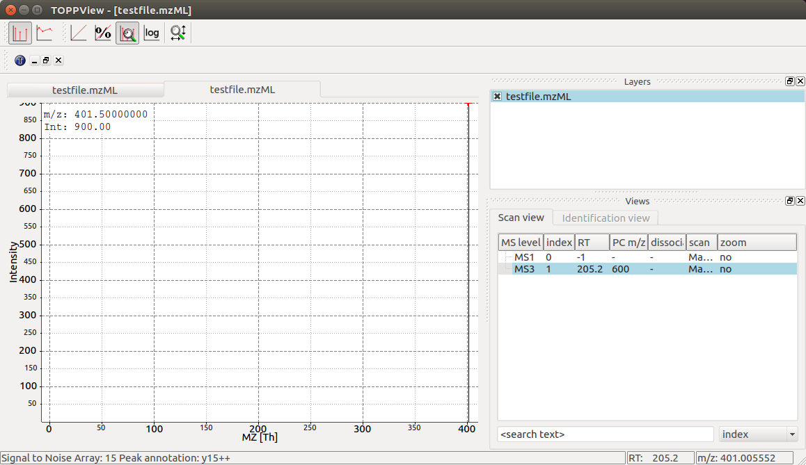
TOPPView displays our mass spectrum with its single peak at \(401.5\ m/z\) and it also correctly displays its retention time at \(205.2\ seconds\) and precursor isolation target of \(600.0/ m/z\). Notice how TOPPView displays the information about the S/N for the peak (S/N = 15) and its annotation as \(\ce{y15++}\) in the status bar below when the user clicks on the peak at \(401.5\ m/z\) as shown in the screenshot.
We can also visualize our mass spectrum from before using the plot_spectrum() function from the
spectrum_utils visualization library:
1import matplotlib.pyplot as plt
2from pyopenms.plotting import plot_spectrum
3
4plot_spectrum(spectrum)
5plt.show()
Chromatogram#
An additional container for raw data is the MSChromatogram container, which
is highly analogous to the MSSpectrum container, but contains an array of
ChromatogramPeak and is derived from ChromatogramSettings:
 1import numpy as np
 2
 3
 4def gaussian(x, mu, sig):
 5    return np.exp(-np.power(x - mu, 2.0) / (2 * np.power(sig, 2.0)))
 6
 7
 8# Create new chromatogram
 9chromatogram = oms.MSChromatogram()
10
11# Set raw data (RT and intensity)
12rt = range(1500, 500, -100)
13i = [gaussian(rtime, 1000, 150) for rtime in rt]
14chromatogram.set_peaks([rt, i])
15
16# Sort the peaks according to ascending retention time
17chromatogram.sortByPosition()
18
19print("Iterate over peaks with getRT() and getIntensity()")
20for p in chromatogram:
21    print(p.getRT(), p.getIntensity())
22
23print("\nIterate more efficiently over peaks with get_peaks()")
24for rt, i in zip(*chromatogram.get_peaks()):
25    print(rt, i)
26
27print("\nAccess an individual peak by index")
28print(chromatogram[2].getRT(), chromatogram[2].getIntensity())
29
30# Add meta information to the chromatogram
31chromatogram.setNativeID("Trace XIC@405.2")
32
33# Store a precursor ion for the chromatogram
34p = oms.Precursor()
35p.setIsolationWindowLowerOffset(1.5)
36p.setIsolationWindowUpperOffset(1.5)
37p.setMZ(405.2)  # isolation at 405.2 +/- 1.5 Th
38p.setActivationEnergy(40)  # 40 eV
39p.setCharge(2)  # 2+ ion
40p.setMetaValue("description", chromatogram.getNativeID())
41p.setMetaValue("peptide_sequence", chromatogram.getNativeID())
42chromatogram.setPrecursor(p)
43
44# Also store a product ion for the chromatogram (e.g. for SRM)
45p = oms.Product()
46p.setMZ(603.4)  # transition from 405.2 -> 603.4
47chromatogram.setProduct(p)
48
49# Store as mzML
50exp = oms.MSExperiment()
51exp.addChromatogram(chromatogram)
52oms.MzMLFile().store("testfile3.mzML", exp)
53
54# Visualize the resulting data using matplotlib
55import matplotlib.pyplot as plt
56
57for chrom in exp.getChromatograms():
58    retention_times, intensities = chrom.get_peaks()
59    plt.plot(retention_times, intensities, label=chrom.getNativeID())
60
61plt.xlabel("time (s)")
62plt.ylabel("intensity (cps)")
63plt.legend()
64plt.show()
Iterate over peaks with getRT() and getIntensity()
600.0 0.028565499931573868
700.0 0.1353352814912796
800.0 0.4111122786998749
900.0 0.8007373809814453
1000.0 1.0
1100.0 0.8007373809814453
1200.0 0.4111122786998749
1300.0 0.1353352814912796
1400.0 0.028565499931573868
1500.0 0.003865920240059495

Iterate more efficiently over peaks with get_peaks()
600.0 0.0285655
700.0 0.13533528
800.0 0.41111228
900.0 0.8007374
1000.0 1.0
1100.0 0.8007374
1200.0 0.41111228
1300.0 0.13533528
1400.0 0.0285655
1500.0 0.0038659202

Access an individual peak by index
800.0 0.4111122786998749
This shows how the MSExperiment class can hold mass spectra as well as chromatograms .
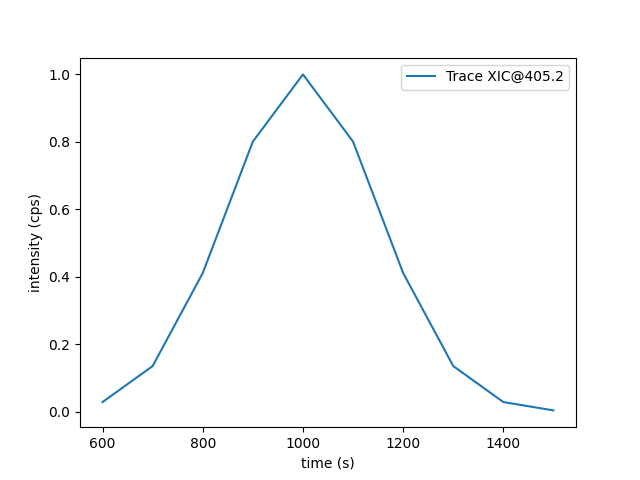
Again we can visualize the resulting data using TOPPView using its chromatographic viewer capability, which shows the peak over retention time:
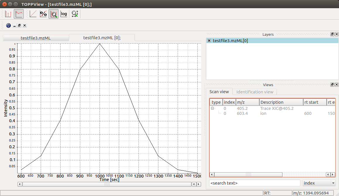
Note how the annotation using precursor and production mass of our XIC chromatogram is displayed in the viewer.
We can also visualize the resulting data using matplotlib. Here we can plot every
chromatogram in our MSExperiment and label it with it’s native ID.
LC-MS/MS Experiment#
In OpenMS, LC-MS/MS injections are represented as so-called peak maps (using
the MSExperiment class), which we have already encountered above. The
MSExperiment class can hold a list of MSSpectrum object (as well as a
list of MSChromatogram objects, see below). The MSExperiment object
holds such peak maps as well as meta-data about the injection. Access to
individual mass spectra is performed through getSpectrum() and
getChromatogram().
In the following code, we create an MSExperiment and populate it with
several mass spectra:
 1# The following examples creates an MSExperiment which holds six
 2# MSSpectrum instances.
 3exp = oms.MSExperiment()
 4for i in range(6):
 5    spectrum = oms.MSSpectrum()
 6    spectrum.setRT(i)
 7    spectrum.setMSLevel(1)
 8    for mz in range(500, 900, 100):
 9        peak = oms.Peak1D()
10        peak.setMZ(mz + i)
11        peak.setIntensity(100 - 25 * abs(i - 2.5))
12        spectrum.push_back(peak)
13    exp.addSpectrum(spectrum)
14
15# Iterate over spectra
16for i_spectrum, spectrum in enumerate(exp, start=1):
17    print("Spectrum {i:d}:".format(i=i_spectrum))
18    for peak in spectrum:
19        print(spectrum.getRT(), peak.getMZ(), peak.getIntensity())
Spectrum 1:
0.0 500.0 37.5
0.0 600.0 37.5
0.0 700.0 37.5
0.0 800.0 37.5
Spectrum 2:
1.0 501.0 62.5
1.0 601.0 62.5
1.0 701.0 62.5
1.0 801.0 62.5
Spectrum 3:
2.0 502.0 87.5
2.0 602.0 87.5
2.0 702.0 87.5
2.0 802.0 87.5
Spectrum 4:
3.0 503.0 87.5
3.0 603.0 87.5
3.0 703.0 87.5
3.0 803.0 87.5
Spectrum 5:
4.0 504.0 62.5
4.0 604.0 62.5
4.0 704.0 62.5
4.0 804.0 62.5
Spectrum 6:
5.0 505.0 37.5
5.0 605.0 37.5
5.0 705.0 37.5
5.0 805.0 37.5
In the above code, we create six instances of MSSpectrum (line 4), populate
it with three peaks at \(500\), \(900\) and \(100\) m/z and append them to the
MSExperiment object (line 13). We can easily iterate over the mass spectra in
the whole experiment by using the intuitive iteration on lines 16-19 or we can
use list comprehensions to sum up intensities of all mass spectra that fulfill
certain conditions:
 1# Sum intensity of all spectra between RT 2.0 and 3.0
 2print(
 3    sum(
 4        [
 5            p.getIntensity()
 6            for s in exp
 7            if s.getRT() >= 2.0 and s.getRT() <= 3.0
 8            for p in s
 9        ]
10    )
11)
700.0
We could store the resulting experiment containing the six mass spectra as mzML
using the MzMLFile object:
1# Store as mzML
2oms.MzMLFile().store("testfile2.mzML", exp)
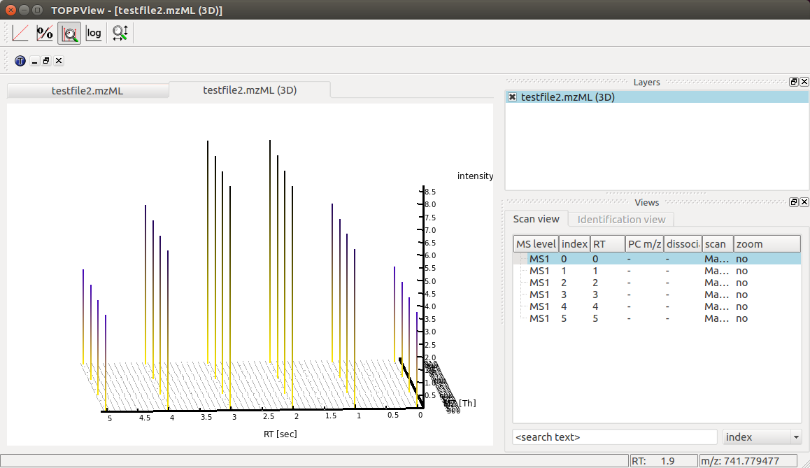
Again we can visualize the resulting data using TOPPView using its 3D viewer capability, which shows the six scans over retention time where the traces first increase and then decrease in intensity:
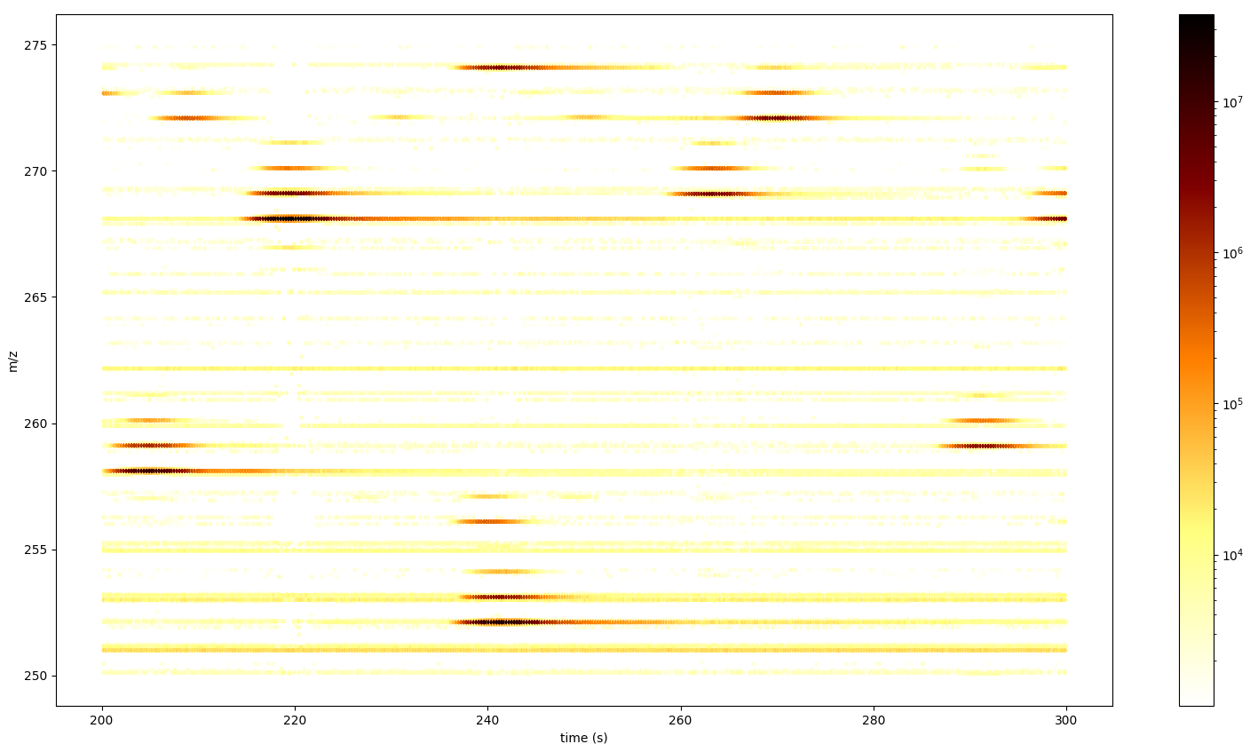
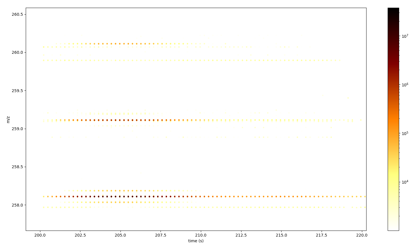
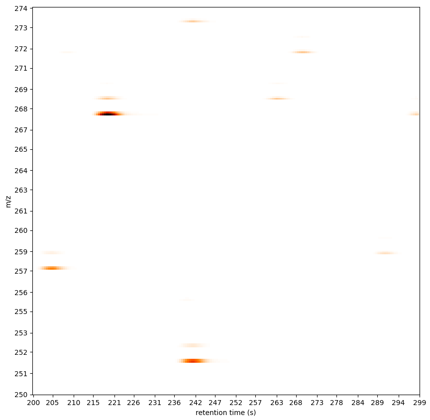
Alternatively we can visualize our data directly with Python. For smaller data sets
we can use matplotlib to generate a 2D scatter plot with the peak intensities
represented by a colorbar. With this plot we can zoom in and inspect our data in more detail.
The following example figures were generated using a mzML file provided by OpenMS.
 1import numpy as np
 2import matplotlib.pyplot as plt
 3import matplotlib.colors as colors
 4
 5
 6def plot_spectra_2D(exp, ms_level=1, marker_size=5):
 7    exp.updateRanges()
 8    for spec in exp:
 9        if spec.getMSLevel() == ms_level:
10            mz, intensity = spec.get_peaks()
11            p = intensity.argsort()  # sort by intensity to plot highest on top
12            rt = np.full([mz.shape[0]], spec.getRT(), float)
13            plt.scatter(
14                rt,
15                mz[p],
16                c=intensity[p],
17                cmap="afmhot_r",
18                s=marker_size,
19                norm=colors.LogNorm(
20                    exp.getMinIntensity() + 1, exp.getMaxIntensity()
21                ),
22            )
23    plt.clim(exp.getMinIntensity() + 1, exp.getMaxIntensity())
24    plt.xlabel("time (s)")
25    plt.ylabel("m/z")
26    plt.colorbar()
27    plt.show()  # slow for larger data sets
28
29
30from urllib.request import urlretrieve
31
32gh = "https://raw.githubusercontent.com/OpenMS/OpenMS/develop/doc/pyopenms"
33urlretrieve(gh + "/src/data/FeatureFinderMetaboIdent_1_input.mzML", "test.mzML")
34
35exp = oms.MSExperiment()
36oms.MzMLFile().load("test.mzML", exp)
37
38plot_spectra_2D(exp)
For larger data sets this will be too slow since every individual peak gets displayed.
However, we can use BilinearInterpolation which produces an overview image of our mass spectra.
This can be useful for a brief visual inspection of your sample in quality control.
 1import numpy as np
 2import matplotlib.pyplot as plt
 3
 4
 5def plot_spectra_2D_overview(experiment):
 6    rows = 200.0
 7    cols = 200.0
 8    exp.updateRanges()
 9
10    bilip = oms.BilinearInterpolation()
11    tmp = bilip.getData()
12    tmp.resize(int(rows), int(cols))
13    bilip.setData(tmp)
14    bilip.setMapping_0(0.0, exp.getMinRT(), rows - 1, exp.getMaxRT())
15    bilip.setMapping_1(0.0, exp.getMinMZ(), cols - 1, exp.getMaxMZ())
16    for spec in exp:
17        if spec.getMSLevel() == 1:
18            mzs, ints = spec.get_peaks()
19            rt = spec.getRT()
20            for i in range(0, len(mzs)):
21                bilip.addValue(rt, mzs[i], ints[i])
22
23    data = np.ndarray(shape=(int(cols), int(rows)), dtype=np.float64)
24    for i in range(int(rows)):
25        for j in range(int(cols)):
26            data[i][j] = bilip.getData().getValue(i, j)
27
28    plt.imshow(np.rot90(data), cmap="gist_heat_r")
29    plt.xlabel("retention time (s)")
30    plt.ylabel("m/z")
31    plt.xticks(
32        np.linspace(0, int(rows), 20, dtype=int),
33        np.linspace(exp.getMinRT(), exp.getMaxRT(), 20, dtype=int),
34    )
35    plt.yticks(
36        np.linspace(0, int(cols), 20, dtype=int),
37        np.linspace(exp.getMinMZ(), exp.getMaxMZ(), 20, dtype=int)[::-1],
38    )
39    plt.show()
40
41
42plot_spectra_2D_overview(exp)
Example: Precursor Purity#
When an MS2 spectrum is generated, the precursor from the MS1 spectrum is gathered, fragmented and measured. In practice, the instrument gathers the ions in a user-defined window around the precursor m/z - the so-called precursor isolation window.
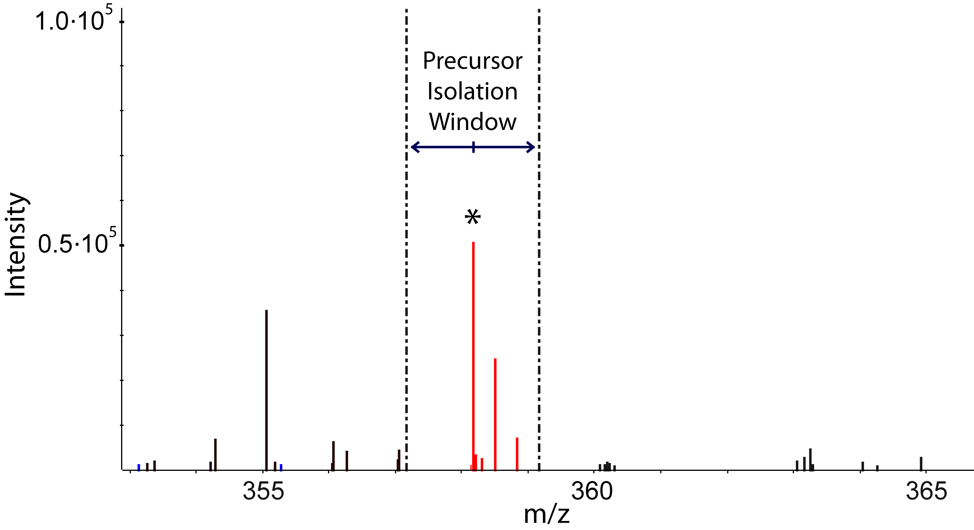
In some cases, the precursor isolation window contains contaminant peaks from other analytes. Depending on the analysis requirements, this can lead to issues in quantification for example, for isobaric experiments.
Here, we can assess the purity of the precursor to filter spectra with a score below our expectation.
 1from urllib.request import urlretrieve
 2
 3gh = "https://raw.githubusercontent.com/OpenMS/OpenMS/develop/doc/pyopenms"
 4urlretrieve(
 5    gh + "/src/data/PrecursorPurity_input.mzML", "PrecursorPurity_input.mzML"
 6)
 7
 8exp = oms.MSExperiment()
 9oms.MzMLFile().load("PrecursorPurity_input.mzML", exp)
10
11# for this example, we check which are MS2 spectra and choose one of them
12for i, element in enumerate(exp):
13    print(str(i) + ": MS" + str(element.getMSLevel()))
14
15# get the precursor information from the MS2 spectrum at index 3
16ms2_precursor = exp[3].getPrecursors()[0]
17
18# get the previous recorded MS1 spectrum
19isMS1 = False
20i = 3  # start at the index of the MS2 spectrum
21while isMS1 == False:
22    if exp[i].getMSLevel() == 1:
23        isMS1 = True
24    else:
25        i -= 1
26
27ms1_spectrum = exp[i]
28
29# calculate the precursor purity in a 10 ppm precursor isolation window
30purity_score = oms.PrecursorPurity().computePrecursorPurity(
31    ms1_spectrum, ms2_precursor, 10, True
32)
33
34print("\nPurity scores")
35print("total:", purity_score.total_intensity)  # 9098343.890625
36print("target:", purity_score.target_intensity)  # 7057944.0
37print("signal proportion:", purity_score.signal_proportion)  # 0.7757394186070014
38print("target peak count:", purity_score.target_peak_count)  # 1
39print("interfering peak count:", purity_score.interfering_peak_count)  # 4
0: MS1
1: MS2
2: MS2
3: MS2
4: MS2
5: MS2
6: MS1

Purity scores
total: 9098343.890625
target: 7057944.0
signal proportion: 0.7757394186070014
target peak count: 1
interfering peak count: 4
We could assess that we have four other non-isotopic peaks apart from our precursor and its isotope peaks within our precursor isolation window. The signal of the isotopic peaks correspond to roughly 78% of all intensities in the precursor isolation window.
Example: Filtering Mass Spectra#
Here we will look at some code snippets that might come in handy when dealing with mass spectra data.
But first, we will load some test data:
1gh = "https://raw.githubusercontent.com/OpenMS/OpenMS/develop/doc/pyopenms"
2urlretrieve(gh + "/src/data/tiny.mzML", "test.mzML")
3
4inp = oms.MSExperiment()
5oms.MzMLFile().load("test.mzML", inp)
Filtering Mass Spectra by MS Level#
We will filter the data from test.mzML file by only retaining
mass spectra that are not MS1 spectra
(e.g. MS2, MS3 or MSn spectra):
1filtered = oms.MSExperiment()
2for s in inp:
3    if s.getMSLevel() > 1:
4        filtered.addSpectrum(s)
5
6# 'filtered' now only contains spectra with MS level >= 2
Alternatively, we can choose to load only spectra of a certain level using PeakFileOptions, which is even more efficient since
unwanted data is not even loaded into memory.
 1# Create a PeakFileOptions object
 2options = oms.PeakFileOptions()
 3options.setMSLevels([2])  # Load only MS level 2
 4
 5# Load the mzML file with the specified options
 6mzml = oms.MzMLFile()
 7mzml.setOptions(options)  # Apply the options
 8mzml.load("test.mzML", filtered)
 9
10# 'filtered' now only contains spectra with MS level == 2
Now exp contains only MS level 2 spectra
Filtering by Scan Number#
We could also use a list of scan numbers as filter criterion to only retain a list of MS scans we are interested in:
1scan_nrs = [0, 2, 5, 7]
2
3filtered = oms.MSExperiment()
4for k, s in enumerate(inp):
5    if k in scan_nrs:
6        filtered.addSpectrum(s)
Note: the scan numbers are the index of the respective spectra in the data file (mzML). This may not be identical to the vendor scan number, especially if the data has been sliced/filtered before.
Advanced Filtering of NativeID via SpectrumLookup#
To find a spectrum using their original scan number from their native ID we can use SpectrumLookup:
 1lookup = oms.SpectrumLookup()
 2
 3## now, we need to define how to extract the vendor scan number from the 'id' attribute in mzML:
 4# Bruker may have:
 5# <spectrum index="0" id="scan=19" defaultArrayLength="15">
 6# thus we can use (this would also work for Thermo native IDs)
 7lookup.readSpectra(inp, "scan=(?<SCAN>\d+)")       ## required: creates an internal look-up table
 8
 9vendor_scan_nrs = [19, 21]  ## our test.mzML contains 4 spectra, starting at scan=19
10
11filtered = oms.MSExperiment()  ## our result, with all spectra we were looking for
12for v_scan_nr in vendor_scan_nrs:
13  filtered.addSpectrum(inp[lookup.findByScanNumber(v_scan_nr)])
14
15filtered.size()         ## prints '2'
16filtered.updateRanges() ## make sure RT and m/z ranges are up to date
Filtering Mass Spectra and Peaks#
Suppose we are interested in only in a small m/z window of our fragment ion mass spectra. We can easily filter our data accordingly:
 1mz_start = 6.0
 2mz_end = 12.0
 3filtered = oms.MSExperiment()
 4for s in inp:
 5    if s.getMSLevel() > 1:
 6        filtered_mz = []
 7        filtered_int = []
 8        for mz, i in zip(*s.get_peaks()):
 9            if mz > mz_start and mz < mz_end:
10                filtered_mz.append(mz)
11                filtered_int.append(i)
12        s.set_peaks((filtered_mz, filtered_int))
13        filtered.addSpectrum(s)
14
15# filtered only contains only fragment spectra with peaks in range [mz_start, mz_end]
For this simple example, you can achieve the same thing using PeakFileOptions when loading the data:
 1# Create a PeakFileOptions object
 2options = oms.PeakFileOptions()
 3options.setMSLevels([2])  # Load only MS level 2
 4options.setMZRange(oms.DRange1(oms.DPosition1(mz_start),oms.DPosition1(mz_end)))
 5
 6# Load the mzML file with the specified options
 7mzml = oms.MzMLFile()
 8mzml.setOptions(options)  # Apply the options
 9mzml.load("test.mzML", filtered)
10
11# 'filtered' now only contains spectra with MS level == 2, and each spectrum has peaks with m/z values between 6-12
Note that in a real-world application, we would set the mz_start and
mz_end parameter to an actual area of interest, for example the area
between 125 and 132 which contains quantitative ions for a TMT experiment.
Similarly we could only retain spectra with a certain retention time or peaks with a certain intensity range.
See PeakFileOptions for details.
For more advanced filtering tasks pyOpenMS provides special algorithm classes. We will take a closer look at some of them in the next section.
Filtering Mass Spectra with TOPP Tools#
We can also use predefined TOPP tools to filter our data. First we need to load in the data:
 1import matplotlib.pyplot as plt
 2from pyopenms.plotting import plot_spectrum, mirror_plot_spectrum
 3
 4gh = "https://raw.githubusercontent.com/OpenMS/OpenMS/develop/doc/pyopenms"
 5urlretrieve(
 6    gh + "/src/data/YIC(Carbamidomethyl)DNQDTISSK.mzML", "observed.mzML"
 7)
 8
 9exp = oms.MSExperiment()
10# Load mzML file and obtain spectrum for peptide YIC(Carbamidomethyl)DNQDTISSK
11oms.MzMLFile().load("observed.mzML", exp)
12
13# Get first spectrum
14spectra = exp.getSpectra()
15observed_spectrum = spectra[0]
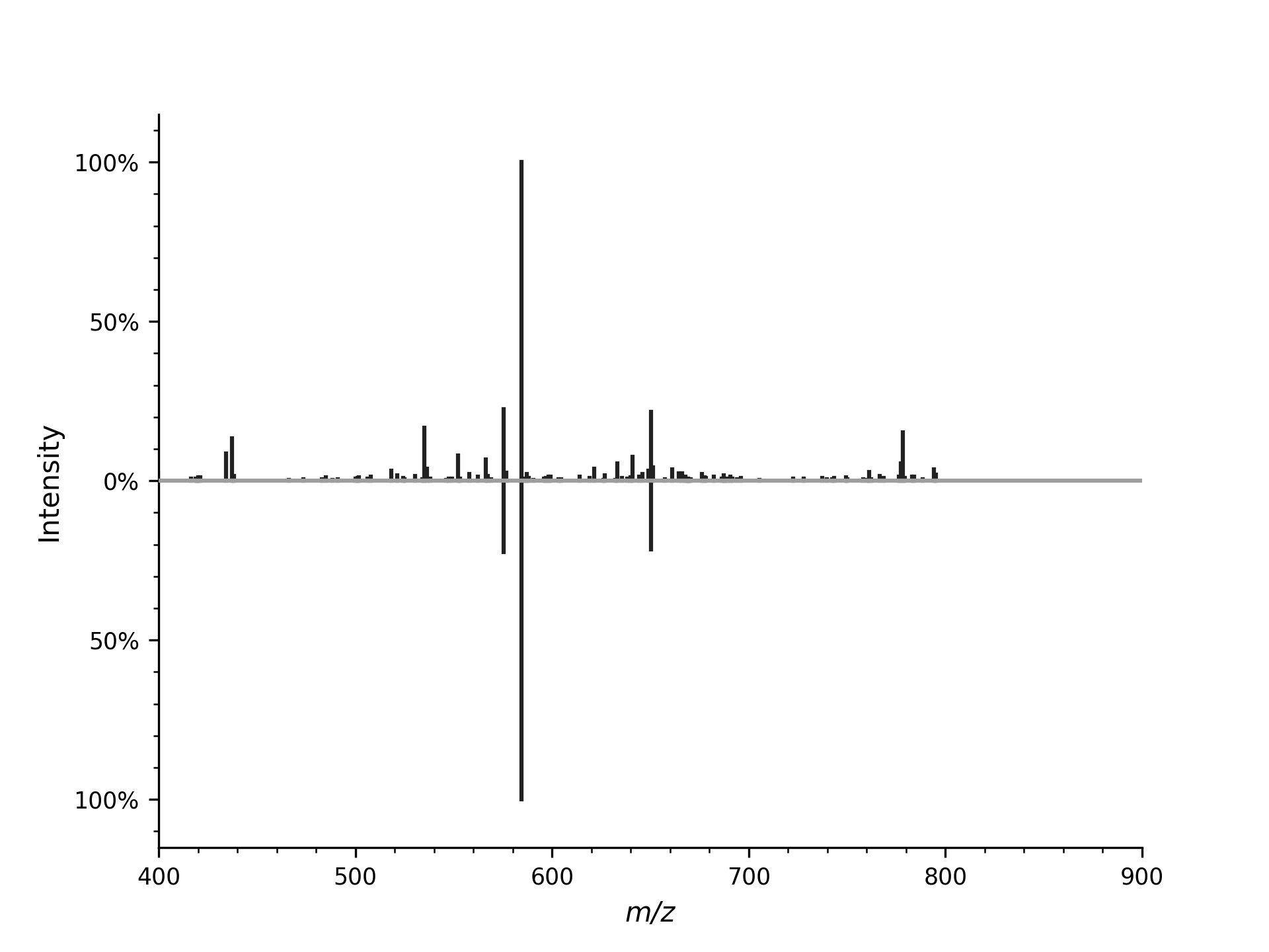
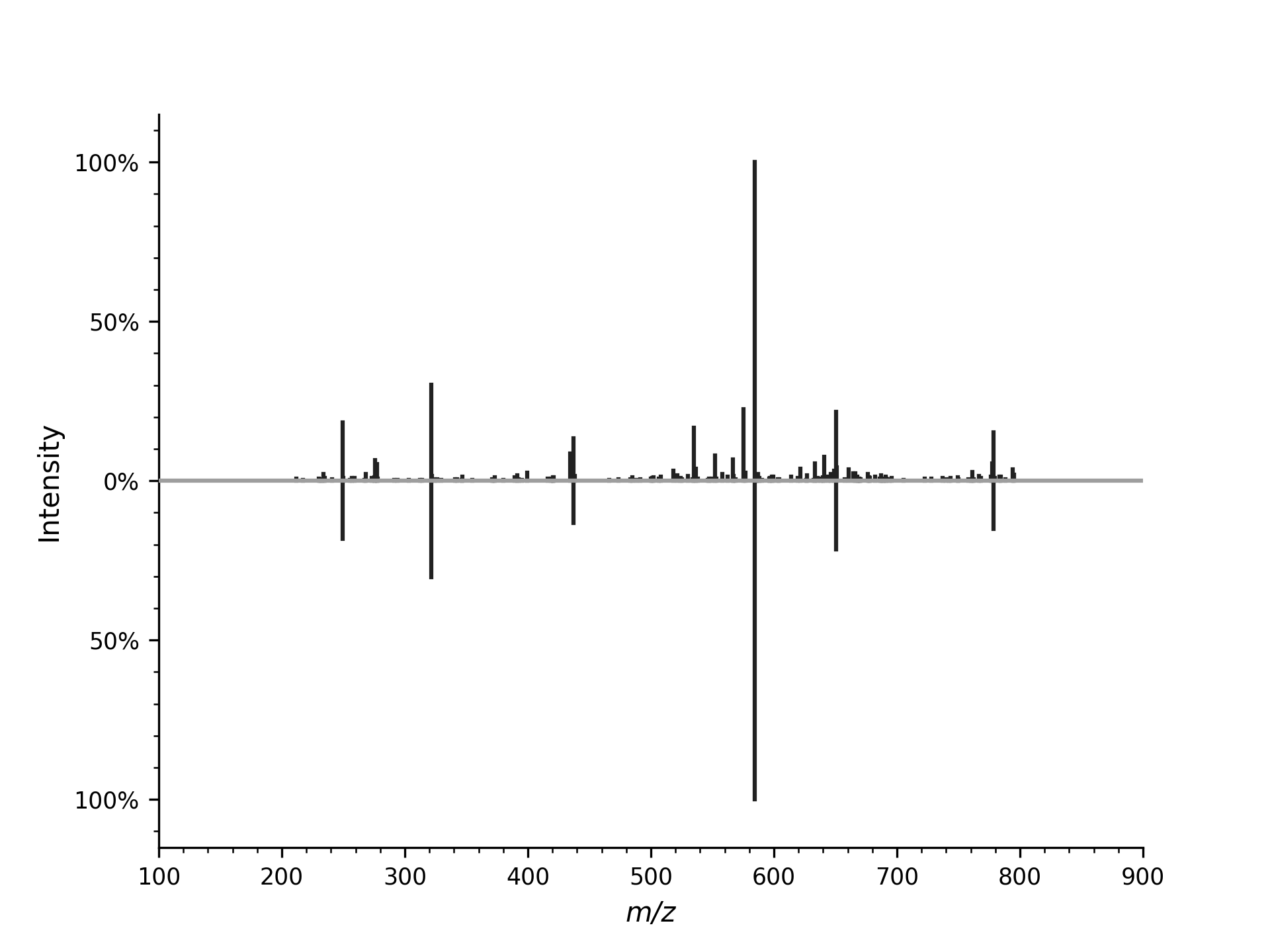
The WindowMower tool can be used to remove peaks in a sliding or jumping window. The window size,
number of highest peaks to keep and move type can be set with a Param object
 1from copy import deepcopy
 2
 3window_mower_filter = oms.WindowMower()
 4
 5# Copy the original spectrum
 6mowed_spectrum = deepcopy(observed_spectrum)
 7
 8# Set parameters
 9params = oms.Param()
10# Defines the m/z range of the sliding window
11params.setValue("windowsize", 100.0, "")
12# Defines the number of highest peaks to keep in the sliding window
13params.setValue("peakcount", 1, "")
14# Defines the type of window movement: jump (window size steps) or slide (one peak steps)
15params.setValue("movetype", "jump", "")
16
17# Apply window mowing
18window_mower_filter.setParameters(params)
19window_mower_filter.filterPeakSpectrum(mowed_spectrum)
20
21# Visualize the resulting data together with the original spectrum
22mirror_plot_spectrum(observed_spectrum, mowed_spectrum)
23plt.show()
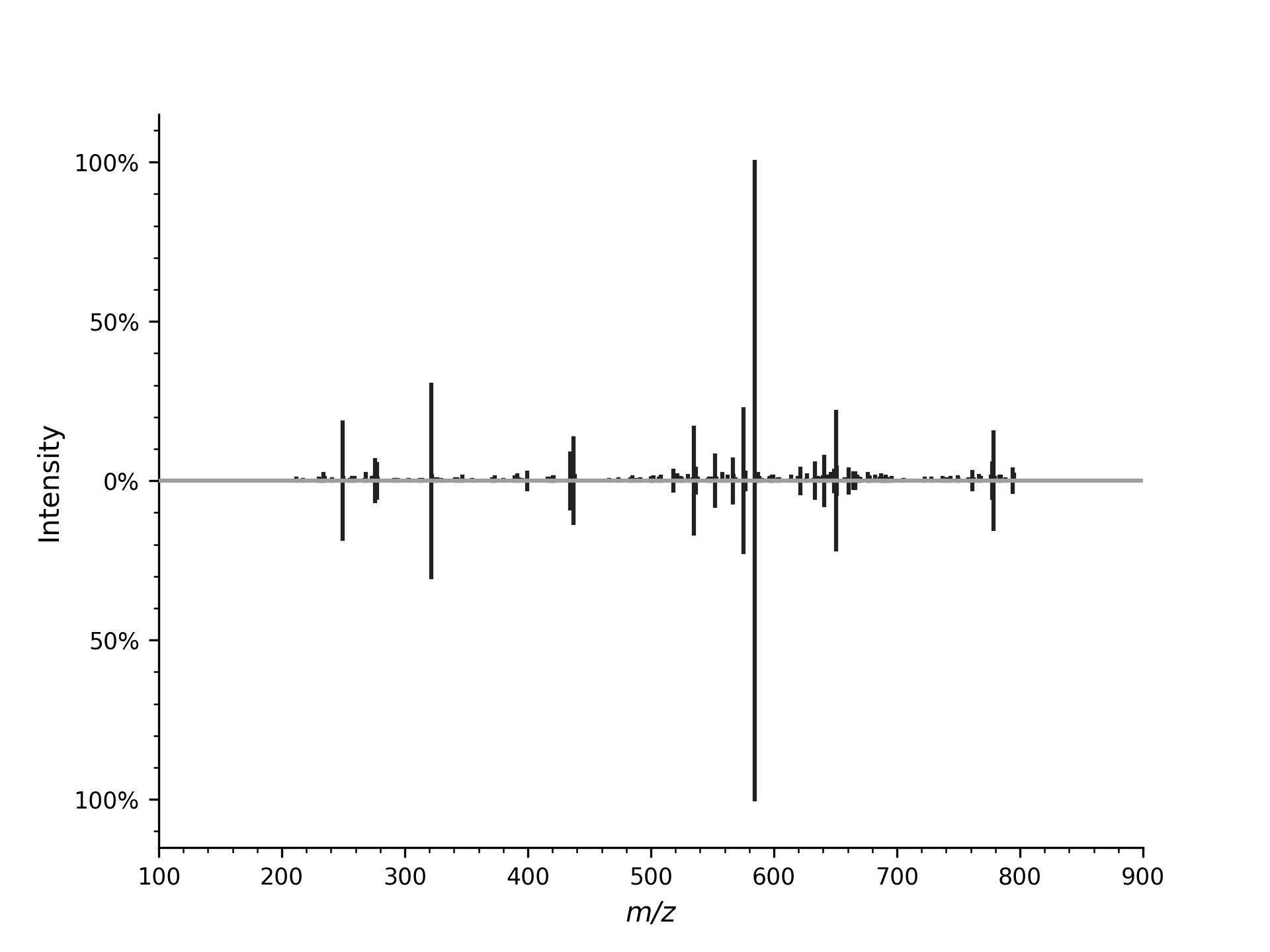
Noise can be easily removed with ThresholdMower by setting a threshold value for the intensity of peaks
and cutting off everything below.
 1# Copy spectrum
 2threshold_mower_spectrum = deepcopy(observed_spectrum)
 3
 4threshold_mower_filter = oms.ThresholdMower()
 5
 6# Set parameters
 7params = oms.Param()
 8params.setValue("threshold", 20.0, "")
 9
10# Apply threshold mowing
11threshold_mower_filter.setParameters(params)
12threshold_mower_filter.filterPeakSpectrum(threshold_mower_spectrum)
13
14mirror_plot_spectrum(observed_spectrum, threshold_mower_spectrum)
15plt.show()
We can also use e.g. NLargest to keep only the N highest peaks in a spectrum.
 1# Copy spectrum
 2nlargest_spectrum = deepcopy(observed_spectrum)
 3
 4nlargest_filter = oms.NLargest()
 5
 6# Set parameters
 7params = oms.Param()
 8params.setValue("n", 4, "")
 9
10# Apply N-Largest filter
11nlargest_filter.setParameters(params)
12nlargest_filter.filterPeakSpectrum(nlargest_spectrum)
13
14mirror_plot_spectrum(observed_spectrum, nlargest_spectrum)
15plt.show()
16# Two peaks are overlapping, so only three peaks are really visible in the plot